A Gentle Introduction to Diffusion Language Models

Abstract

Large Language Models have been the most trending topic in Machine Learning for the past few years. While the majority of models are based on the Autoregressive framework, in which tokens are generated in a left-to-right fashion, recently, advances in Discrete Diffusion have managed to come up with a new any-order framework. These models are known as Diffusion Language Models (DLMs), and in this post, I will briefly guide you through the theoretical and practical foundations of these models.

1. General background

1.1 Transformer recap

Before going on to present DLMs, I want to make a quick recap on the Transformer [1] architecture and causality in Autoregressive models.

As in all modern NLP papers, let's introduce the attention mechanism:

Here, $A_{i,j}$ represents the attention that token $i$ pays to $j$. Intuitively, $\sum_j A_{i,j}=1$. In Autoregressive models (ARMs), we introduce a causal mask, preventing tokens after position $i$ from being seen by token $x_i$. Moreover, the last token at the current sequence $x_n$, encodes the information to predict the next token $x_{n+1}$. Keep these facts in mind as they will no longer be true for DLMs.

1.2 Caching

A big advantage of the causal mask introduced in ARMs is that representations from all previously generated tokens remain fixed. This is due to how we model the attention mask, as we get a plot in a triangle fashion:

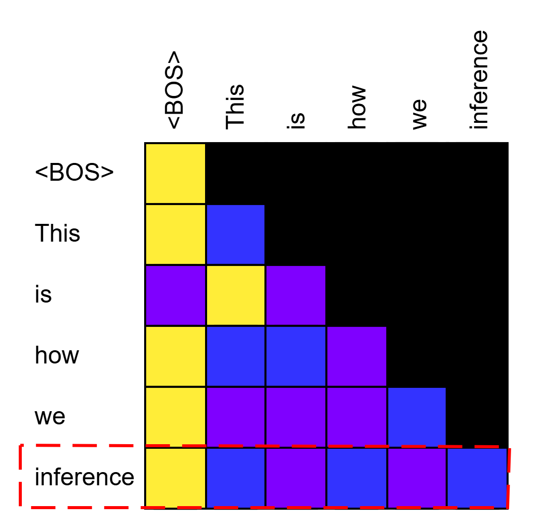
Generating a new token amounts to appending one row to the plot, but how the attention is modelled for all previous $n-1$ tokens remains fixed. As the attention does not change, neither does the weighting by the Value vectors, and therefore, nor does the hidden state of the tokens. This enables efficiency techniques such as KV-caching, because we can cache the Key and Value vectors of all previous tokens and just compute the attention for the newly generated one (note that Query values for old tokens can be safely discarded) without losing quality. This will be another big point of distinction among DLMs and ARMs.

1.3 Autoregressive Language Models

Autoregressive Language Models assume the following factorization of probabilities:

This formulation formally frames what we have introduced before, i.e. "tokens just need to pay attention to tokens coming before them". Training a model amounts to maximizing the likelihood on the training data, or, what is equivalent, reducing the KL-divergence between the model and the data:

Having introduced all these basic principles, we may now move to diffusion-based models.​

2. Diffusion Language Models

2.1 New formulation

DLMs will frame the generation paradigm in a different way. The first paper to translate diffusion into the discrete domain has been [2]. To keep it simple, they define a forward (noising) and backward (denoising) diffusion process. So, the sequence of discrete characters gets corrupted until arriving to a fully-corrupted sequence at $t=T$, while the clean, original sequence is at $t=0$. They define the forward process as:

In the equation, $x_t$ is a one-hot vector with a 1 at the corresponding character of our vocabulary $K$, and $Q_t$ is the transition matrix, modelling how states change from time $t-1$ to $t$. So, what the formula states is how probable it is to go to a new state $x_t$ starting from $x_{t-1}$, considering that we are in a categorical distribution ($K$ states) and that the transition dynamics are governed by $Q_t$. If you got lost, don't worry, we will later see an example. For the rest of this blog I will refer to the Absorbing States formulation, in which there is an absorbing state - call it [MASK] - to which our sequence will converge as we approach $t=T$. This means that we are only concerned in modelling how probable it is for each of the elements of the sequence to turn into this [MASK] state at each step. Formally, to make the jump from the clean sequence $x_0$ to any intermediate step $x_t$, we would compute:

What we basically did is chain all the transitions starting from the beginning. Intuitively, this gets complicated really quick as we scale the number of steps, moreover, it doesn't let us 'directly' jump to any $t$ without materializing all the matrices in the middle. Fortunately, in practice, we don't even deal with matrices, as the transitions are modelled as a linear schedule of each state getting absorbed (note that state is equivalent to saying token), i.e., transitioning to [MASK]:

In some places you will find this equation with just $t$ and no $T$, as it gets formulated assuming that $t \in [0,1]$, which makes it more difficult to define the matrices introduced before.

Our model then will have to reverse this noising process, and so we model the backward transition as ($0\leq s < t \leq T$):

While at first glance there are many things happening, let me decompose each statement. The first row is just forcing unmasked tokens to remain unmasked, which aligns with the training loss, as the model was just trained to predict on unmasked tokens (note that this limitation has been and is being challenged by the research community, as it limits the models' capabilities of improving unmasked tokens based on newer information, see [3], [4], and [5] for some examples).

The second line comes from computing the posterior $q(x^i_s|x^i_t) = \frac{q(x^i_s | x^i_t).q(x^i_s)}{q(x^i_t)}$ when both $x^i_s$ and $x^i_t$ are equal [MASK]. Note that $q(x^i_s | x^i_t)=1$, $q(x^i_s=\text{[MASK]})=q(x^i_s=\text{[MASK]}|x^i_0)=\frac{s}{T}$ and $q(x^i_t=\text{[MASK]})=q(x^i_t=\text{[MASK]}|x^i_0)=\frac{t}{T}$.

The last line is the one calling the model, and it simply weights the remaining probability of the token not being [MASK] at $s$ by the output distribution of our model. It is important to clarify that the model always predicts the state of the token at the initial time $t=0$, and does not model the intermediate possible latent states that the token may assume. New research works on this aspect, trying to align the model trajectories over time, making the denoising process more stable, and therefore easier to accelerate [6].

2.2 Training

To finish with the theory behind DLMs, let's see how the training loss is modelled and what it implies. In DLMs, as in any other diffusion-based model, we don't generate the whole noising process when training our model. Similarly as in [7], we introduced the transition probabilities from $t=0$ to any $t$ to easily get training examples for the model without going through the whole noising chain. The loss ends up being the likelihood that the model correctly predicts all the masked tokens at a certain timestep:

So, what we do during training is sample a random time, mask the corresponding tokens based on our transition dynamics and train the model to correctly predict the state of those tokens before being masked.

2.3 Inference

There are many ways of inferring the model, as there are hyperparameters with which we can play. Before starting the generation, in classical DLMs, we should define the number of denoising steps $T$ and the generation length $L$. This way, what we do is append $L$ [MASK] tokens to our input, and based on some denoising schedule, we will unmask tokens for $T$ iterations. A vanilla DLM denoising process would look like this (unmasking at each step following the transition dynamics introduced in 2.1):

Different models define different ways of unmasking and selecting tokens, adapting the transition probabilities we introduced in 2.1 to their application. In LLaDA [8], for example, they order the confidence score (i.e., the highest probability of the Categorical distribution) of all the masked tokens and unmask only the top-k of them. The parameter k is defined as $k=L/T$, so $L$ has to be a multiple of $T$. As mentioned before, many works are researching how to better infer these models without significant loss in performance, e.g. [9] explores how can we do inference-time scaling by decomposing and selecting a reference sequence that will get improved as we explore different trajectories.

2.4 Practical implications

Before finishing, I want to give some final remarks on the opportunities and current limitations of DLMs. The biggest opportunity that DLMs propose is more efficient when generating the response. By design, they are able to unmask more than one token at the time, and what's more, they can do it in an any-order way, which opens many questions about how language is modelled and how can we extend the models' capabilities. Moreover, the fact that we use a bidirectional attention, as the one in BERT [10] and encoder models, enabling models to modify their previous beliefs about already generated tokens as the sequence progresses. Also, these models enable better controlability of the response in contrast with ARMs, as we can tune the hyperparameters to match our needs or improve performance/speed.

However, most of the aforementioned points are still to be consolidated in the DLM field, as the efficiency that the models provide out-of-the-box is generally worse than that of ARMs (mainly due to the lack of caching, which works like [11] paved the way in this direction, offering a grounded and performant solution). The current community is aiming towards a hybrid architecture that takes the best from both worlds: causality from ARMs, while preserving any-order from DLMs; though, we always face tradeoffs, as by definition, the two concepts are not completely compatible with one another. As for the accuracy and quality of these models, it remains unclear whether they inherently learn better text-relationships compared to ARMs, or the true bottleneck is the Transformer architecture (recent work has shown that DLMs actually learn "faster" in comparison with ARMs, i.e., they need less data to achieve the same performance [12]). Finally, the hyperparameter tuning is a double-edged knife, as it enables greater flexibility, but also puts more complexity in how to tune them correctly, and introduce greater variance in the model's responses.

3. Conclusion

I am not going to do a generic conclusion and will rather keep it short. DLMs have many capabilities that are left to be exploited. Whether these models are better or not at modelling text compared to ARMs remains an open question. Moreover, the big advantages that these models enable are yet to be more fully exploited to provide a suitable replacement for ARMs.

If you liked this post and are interested in DLMs, you can see our work on Attention Sinks [13] where we explore how these models dynamically change the most important token across steps, which sheds light on how we can better KV-cache and discard tokens when modelling long sequences.

References

1. Vaswani, A. et al. (2017). Attention Is All You Need. https://arxiv.org/abs/1706.03762
2. Austin, J. et al. (2023). Structured Denoising Diffusion Models in Discrete State-Spaces. https://arxiv.org/abs/2107.03006
3. Kim, J. et al. (2025). Fine-Tuning Masked Diffusion for Provable Self-Correction. https://arxiv.org/abs/2510.01384
4. Wang, G. et al. (2025). Remasking Discrete Diffusion Models with Inference-Time Scaling. https://arxiv.org/abs/2503.00307
5. Huang, Z. et al. (2025). Don't Settle Too Early: Self-Reflective Remasking for Diffusion Language Models. https://arxiv.org/abs/2509.23653
6. Kim, M. et al. (2025). CDLM: Consistency Diffusion Language Models For Faster Sampling. https://arxiv.org/abs/2511.19269
7. Ho, J. et al. (2020). Denoising Diffusion Probabilistic Models. https://arxiv.org/abs/2006.11239
8. Nie, S. et al. (2025). Large Language Diffusion Models. https://arxiv.org/abs/2502.09992
9. Dang, M. et al. (2025). Inference-Time Scaling of Diffusion Language Models with Particle Gibbs Sampling. https://arxiv.org/abs/2507.08390
10. Devlin, J. et al. (2019). BERT: Pre-training of Deep Bidirectional Transformers for Language Understanding. https://arxiv.org/abs/1810.04805
11. Wu, C. et al. (2025). Fast-dLLM: Training-free Acceleration of Diffusion LLM by Enabling KV Cache and Parallel Decoding. https://arxiv.org/abs/2505.22618
12. Ni, J. et al. (2025). Diffusion Language Models are Super Data Learners. https://arxiv.org/abs/2511.03276
13. Rulli, M. et al. (2025). Attention Sinks in Diffusion Language Models. https://arxiv.org/abs/2510.15731